One Step Diffusion Models

Despite the promising performance of diffusion models on continuous modality generation, one deficiency that is holding them back is their requirement for multi-step denoising processes, which can be computationally expensive. In this article, we examine recent works that aim to build diffusion models capable of performing sampling in one or a few steps.

Background

Diffusion models (DMs), or more broadly speaking, score-matching generative models, have become the de facto framework for building deep generation models. They demonstrate exceptional generation performance, especially on continuous modalities including images, videos, audios, and spatiotemporal data.

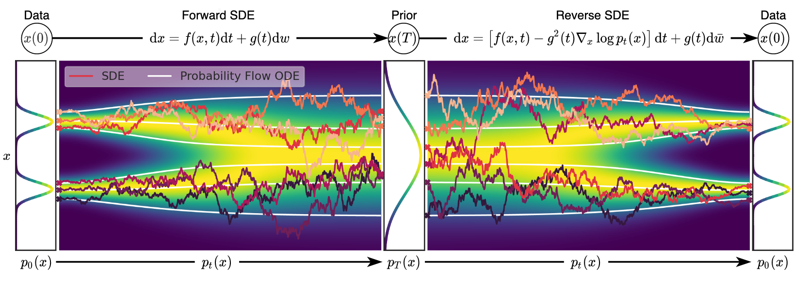
Most diffusion models work by coupling a forward diffusion process and a reverse denoising diffusion process. The forward diffusion process gradually adds noise to the ground truth clean data $X_0$, until noisy data $X_T$ that follows a relatively simple distribution is reached. The reverse denoising diffusion process starts from the noisy data $X_T$, and removes the noise component step-by-step until clean generated data $X_0$ is reached. The reverse process is essentially a Monte-Carlo process, meaning it cannot be parallelized for each generation, which can be inefficient for a process with a large number of steps.

Understanding DMs

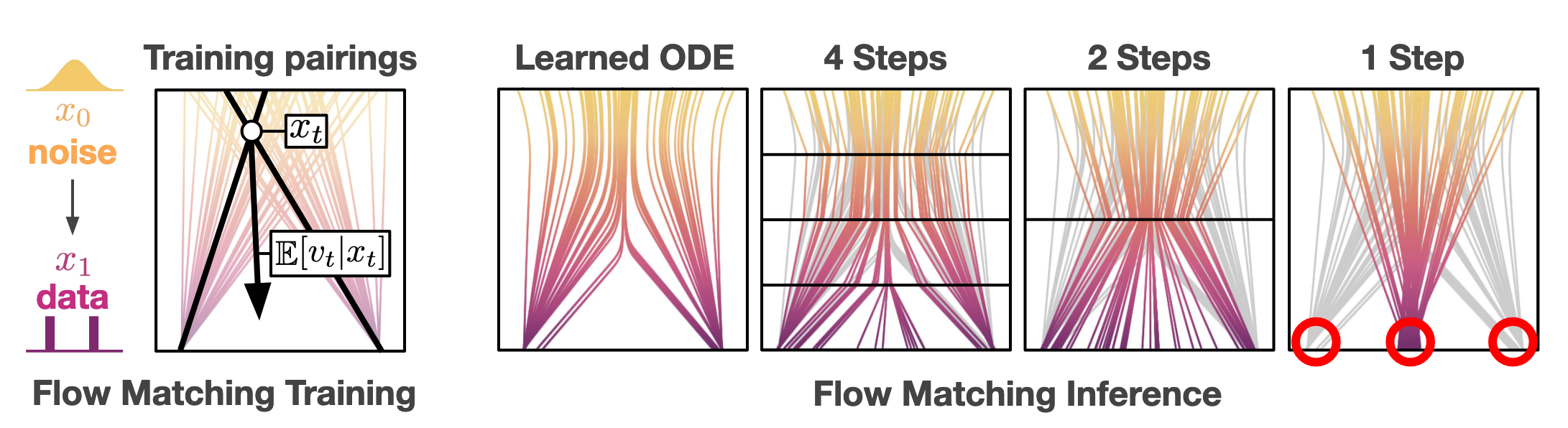
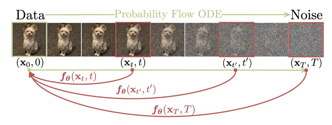
There are many ways to understand how Diffusion Models (DMs) work. One of the most common and intuitive approaches is that a DM learns an ordinary differential equation (ODE) that transforms noise into data. Imagine an ODE vector field between the noise $X_T$ and clean data $X_0$. By training on sufficiently large numbers of timesteps $t\in [0,T]$, a DM is able to learn the vector (tangent) towards the cleaner data $X_{t-\Delta t}$, given any specific timestep $t$ and the corresponding noisy data $X_t$. This idea is easy to illustrate in a simplified 1-dimensional data scenario.

DMs Scale Poorly with Few Steps

Vanilla DDPM, which is essentially a discrete-timestep DM, can only perform the reverse process using the same number of steps it is trained on, typically thousands. DDIM introduces a reparameterization scheme that enables skipping steps during the reverse process of DDPM. Continuous-timestep DMs like Stochastic Differential Equations (SDE) naturally possess the capability of using fewer steps in the reverse process compared to the forward process/training.

Ho, Jain, and Abbeel, “Denoising Diffusion Probabilistic Models.” Song, Meng, and Ermon, “Denoising Diffusion Implicit Models.” Song et al., “Score-Based Generative Modeling through Stochastic Differential Equations.”

Nevertheless, it is observed that their performance typically suffers catastrophic degradation when reducing the number of reverse process steps to single digits.

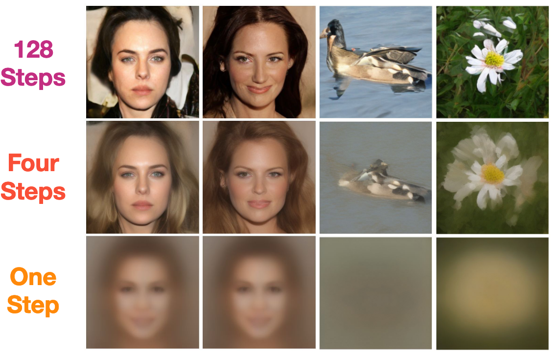
To understand why DMs scale poorly with few reverse process steps, we can return to the ODE vector field perspective of DMs. When the target data distribution is complex, the vector field typically contains numerous intersections. When a given $X_t$ and $t$ is at these intersections, the vector points to the averaged direction of all candidates. This causes the generated data to approach the mean of the training data when only a few reverse process steps are used. Another explanation is that the learned vector field is highly curved. Using only a few reverse process steps means attempting to approximate these curves with polylines, which is inherently difficult.

We will introduce two branches of methods that aim to scale DMs to few or even reverse process steps: distillation-based, which distillates a pre-trained DM into a one-step model; and end-to-end-based, which trains a one-step DM from scratch.

Distallation

Distillation-based methods are also called rectified flow methods. Their idea follows the above insight of "curved ODE vector field": if the curved vectors (flows) are hindering the scaling of reverse process steps, can we try to straighten these vectors so that they are easy to approximate with polylines or even straight lines?

Liu, Gong, and Liu, "Flow Straight and Fast" implements this idea, focusing on learning an ODE that follows straight vectors as much as possible. In the context of continuous time DMs where $T=1$ and and $t\in[0,1]$, suppose the clean data $X_0$ and noise $X_1$ each follows a data distribution, $X_0\sim \pi_0$ and $X_1\sim \pi_1$. The "straight vectors" can be achieved by solving a nonlinear least squares optimization problem: $$\min_{v} \int_{0}^{1} \mathbb{E}\left[\left\|\left(X_{1}-X_{0}\right)-v\left(X_{t}, t\right)\right\|^{2}\right] \mathrm{d} t,$$

$$\quad X_{t}=t X_{1}+(1-t) X_{0}$$

Where $v$ is the vector field of the ODE $dZ_t = v(Z_t,t)dt$.

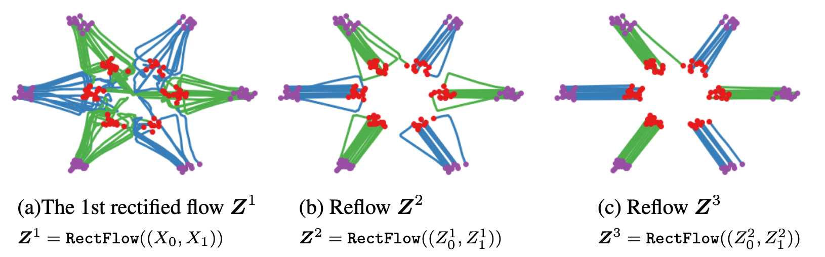
Though straightforward, when the clean data distribution $\pi_0$ is very complicated, the ideal result of completely straight vectors can be hard to achieve. To address this, a "reflow" procedure is introduced. This procedure iteratively trains new rectified flows using data generated by previously obtained flows: $$Z^{(k+1)} = RectFlow((Z_0^k, Z_1^k))$$ This procedure produces increasingly straight flows that can be simulated with very few steps, ideally one step after several iterations.

In practice, distillation-based methods are usually trained in two stages: first train a normal DM, and later distill one-step capabilities into it. This introduces additional computational overhead and complexity.

End-to-end

Compared to distillation-based methods, end-to-end-based methods train a one-step-capable diffusion model (DM) within a single training run. Various techniques are used to implement such methods. We will focus on two of them: consistency models and shortcut models.

Consistency Models

In discrete-timestep diffusion models (DMs), three components in the reverse denoising diffusion process are interchangeable through reparameterization: the noise component $\epsilon_t$ to remove, the less noisy previous step $x_{t-1}$, and the predicted clean sample $x_0$. This interchangeability is enabled by the following equation: $$x_t = \sqrt{\bar{\alpha}_t} \, x_0 + \sqrt{1 - \bar{\alpha}_t} \, \epsilon_t$$ In theory, without altering the fundamental formulation of DMs, the learnable denoiser network can be designed to predict any of these three components. Consistency models (CMs) follow this principle by training the denoiser to specifically predict the clean sample $x_0$. The benefit of this approach is that CMs can naturally scale to perform the reverse process with few steps or even a single step.

Formally, CMs learn a function $f_\theta(x_t,t)$ that maps noisy data $x_t$ at time $t$ directly to the clean data $x_0$, satisfying: $$f_\theta(x_t, t) = f_\theta(x_{t'}, t') \quad \forall t, t'$$ The model must also obey the differential consistency condition: $$\frac{d}{dt} f_\theta(x_t, t) = 0$$ CMs are trained by minimizing the discrepancy between outputs at adjacent times, with the loss function: $$\mathcal{L} = \mathbb{E} \left[ d\left(f_\theta(x_t, t), f_\theta(x_{t'}, t')\right) \right]$$ Similar to continuous-timestep DMs and discrete-timestep DMs, CMs also have continuous-time and discrete-time variants. Discrete-time CMs are easier to train, but are more sensitive to timestep scheduling and suffer from discretization errors. Continuous-time CMs, on the other hand, suffer from instability during training.

For a deeper discussion of the differences between the two variants of CMs, and how to stabilize continuous-time CMs, please refer to Lu and Song, "Simplifying, Stabilizing and Scaling Continuous-Time Consistency Models."

Shortcut Models

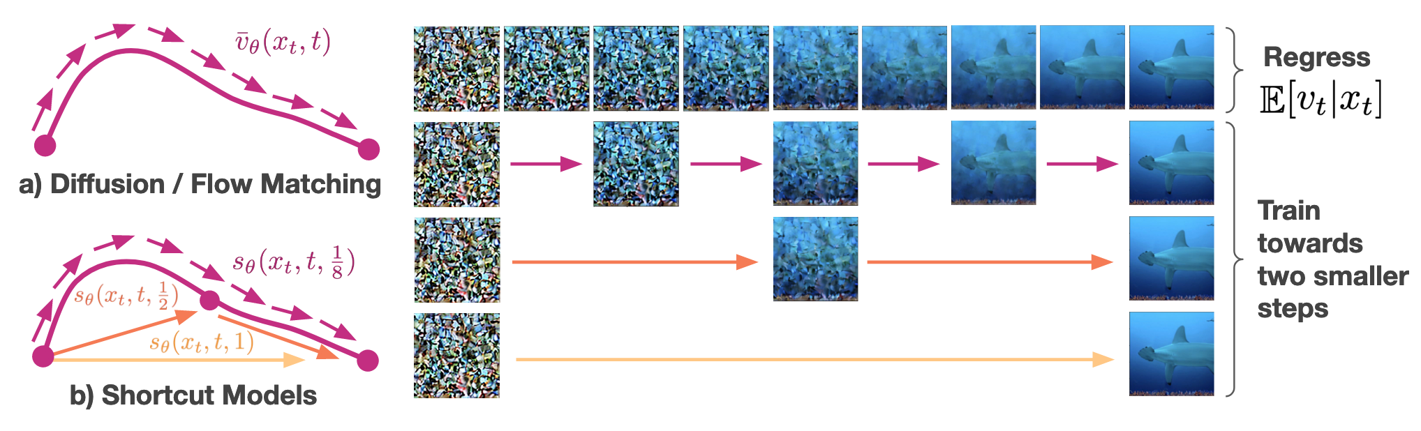
Similar to distillation-based methods, the core idea of shortcut models is inspired by the "curved vector field" problem, but the shortcut models take a different approach to solve it.

Shortcut models are introduced in Frans et al., "One Step Diffusion via Shortcut Models." The paper presents the insight that conventional DMs perform badly when jumping with large step sizes stems from their lack of awareness of the step size they are set to jump forward. Since they are only trained to comply with small step sizes, they are only learning the tangents in the curved vector field, not the "correct direction" when a large step size is used.

Based on this insight, on top of $x_t$ and $t$, shortcut models additionally include step size $d$ as part of the condition for the denoiser network. At small step sizes ($d\rightarrow 0$), the model behaves like a standard flow-matching model, learning the expected tangent from noise to data. For larger step sizes, the model learns that one large step should equal two consecutive smaller steps (self-consistency), creating a binary recursive formulation. The model is trained by combining the standard flow matching loss when $d=0$ and the self-consistency loss when $d>0$: $$\mathcal{L} = \mathbb{E} [ \underbrace{\| s_\theta(x_t, t, 0) - (x_1 - x_0)\|^2}_{\text{Flow-Matching}} +$$

$$\underbrace{\|s_\theta(x_t, t, 2d) - \mathbf{s}_{\text{target}}\|^2}_{\text{Self-Consistency}}],$$

$$\quad \mathbf{s}_{\text{target}} = s_\theta(x_t, t, d)/2 + s_\theta(x'_{t+d}, t + d, d)/2 \quad$$

$$\text{and} \quad x'_{t+d} = x_t + s_\theta(x_t, t, d)d$$

Both consistency models and shortcut models can be seamlessly scaled between one-step and multi-step generation to balance quality and efficiency.